Customers are the biggest asset of any business. For example, if you are an e-commerce company trying to maximize customer incentivization, understanding your customer-base is essential to helping you make better customer recommendations. If you are a next-generation sequencing company trying to minimize specimen collection, understanding your customer-base is essential to making better operational decisions.
The simplest model for understanding customer decisions is the Markov chain. Although the math behind Markov chains can be quite involved and deep, they are quite easy to understand and use, and Setosa has a great primer on the subject. Here, I want to demonstrate the full-power of using Markov chains and Sankey diagrams in summarizing the bulk behavior of your entire customer-base in just a few numbers and an intuitive visualization. In the absence of data, instead of taking real data and simulating it using its statistics, I take the reverse approach of starting with the simulation and verifying it has the expected statistics.
The Problem Statement
Suppose you spend a day at Disneyland and station people at Space Mountain (SM), Indiana Jones Adventure (IJA), and Haunted Mansion (HM). When they entered the park, they were registered with a customer_id, and as they come out of each ride, you record them until they opt out of your study.
Three rows of your database might look like this:
| order_id | customer_id | order_num | order_date | item |
|---|---|---|---|---|
| 1931 | 1 | 0 | 2020-11-24 10:54:19 | Haunted Mansion |
| 4040 | 2 | 0 | 2020-11-24 11:31:51 | Indiana Jones Adventure |
| 6444 | 2 | 1 | 2020-11-24 12:40:51 | Space Mountain |
This would be the data returned by the super simple SQL query:
SELECT order_id, customer_id, order_num, order_date, item
FROM orders
ORDER BY customer_id, order_id;
If you work at a company that deals with customers, chances are you have some variation of this table in a SQL database somewhere. If so, the techniques I will cover will can easily be adapted for your use-case.
About Markov Chains
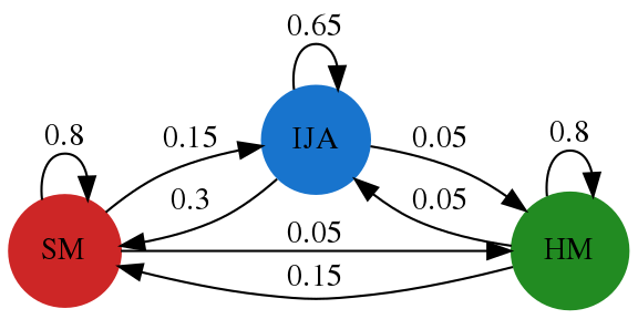
The Markov chain is a model in which a system is assigned an initial state and assumed to transition from state to state randomly according to pre-defined probabilities. These probabilities are typically summarized using a state transition diagram like the one below, which we will be using later.
Simple Markov chains typically make three simple assumptions:
- All customers make their choices independently.
- Customers make their next choice only based on their current choice.
- Customer choices do not vary over time.
Even if these assumptions are not met, data simulated by a Markov chain can look uncannily similar to real data, which makes it an extremely powerful as a tool for building other tools before real data becomes available. For example, the code I wrote for plotting Sankey diagrams was built upon this simulated data and will work for any real customer data as well.
Simulations
Python has a module called SimPy that makes simulations easy. SimPy’s Environment class manages the simulation time, and all you have to do is define processes in the form of while loops that yield timeouts to the Environment during the run. The simulation then runs until the specified time.
To demonstrate a very simple example, consider the following processes:
class FirstProcess:
    def __init__(self, env):
        self.env = env

    def run(self):
        while True:
            print(f'First Process: {self.env.now}')
            yield self.env.timeout(1)

class SecondProcess:
    def __init__(self, env):
        self.env = env

    def run(self):
        while True:
            print(f'Second Process: {self.env.now}')
            yield self.env.timeout(2)
If I instantiate first_process = FirstProcess(env) and run the while loop, each iteration will yield env.timeout(1) to the SimPy Environment. Let’s see how this works:
import simpy

env = simpy.Environment()

first_process = FirstProcess(env)
env.process(first_process.run())

second_process = SecondProcess(env)
env.process(second_process.run())

env.run(until=5)
The output of the above code is:
First Process: 0
Second Process: 0
First Process: 1
Second Process: 2
First Process: 2
First Process: 3
Second Process: 4
First Process: 4
Simple, right?
Simulate Customers using Markov Chains
The name of the game here is to turn the above simulation into a Markov chain. To accomplish this, we can view a Customer as a process whose purpose is to make_choices at specified time intervals. Using the blueprint from FirstProcess, we can define our basic customer as:
class Customer:
    def __init__(self, env):
        self.env = env

    def make_choices(self):
        while True:
            yield self.env.timeout(1)
Of course, we’re going to want to collect a lot more attributes on the customer so that we can retrieve them while the simulation runs.
- Every customer has a unique
customer_id, which we’ll generate externally. - To keep track of each customer’s choices, let’s add
current_choiceandcurrent_timeattributes. - To keep track of time, let’s keep track of
start_timeso we can convert SimPy’senv.nowto adatetimeobject. - Finally, let’s arbitrarily say that our customer starts at Space Mountain.
Our initial Customer now looks like this:
class Customer:
    def __init__(self, env, customer_id):

        self.env = env

        self.customer_id = customer_id
        self.order_num = 0
        self.start_time = dt.datetime(2020, 11, 24, 10, 0, 0)
        self.current_time = dt.datetime(2020, 11, 24, 10, 15, 0)
        self.current_choice = 'Space Mountain'

    def make_choices(self):
        while True:
            yield self.env.timeout(1)
Not all of our customers will have their first_choice() be Space Mountain or arrive at the same current_time. To better approximate reality, let’s initialize the first_choice() randomly according to predefined distributions and specify that the customer can arrive any time between 10:15 am and 12:00 pm. Let’s also advance the env clock to start at the customer’s first current_time in minutes and truncate the timestamp so we’re not collecting millisecond data. Finally, let’s collect the results so we can examine the output as we build up the simulation. Our Customer now looks like:
import datetime as dt
import numpy as np


class Customer:
    def __init__(self, env, results, customer_id):

        self.env = env
        self.results = results

        self.customer_id = customer_id
        self.order_num = 0

        # generate timestamps
        self.earliest_start = dt.datetime(2020, 11, 24, 10, 15, 0)
        self.latest_start = dt.datetime(2020, 11, 24, 12, 0, 0)
        self.current_time = truncate_timestamp(self.first_timestamp())

        # starting conditions
        self.choices = ['Space Mountain', 'Indiana Jones Adventure', 'Haunted Mansion']
        self.initial_weights = [0.50, 0.30, 0.20]
        self.current_choice = self.first_choice()

        # model parameters
        self.env_start = dt.datetime(2020, 11, 24, 10, 0, 0)

    def make_choices(self):

        yield self.align_env_clock()
        while True:

            # record the result
            self.results.append({'customer_id': self.customer_id,
                                 'order_num': self.order_num,
                                 'order_date': self.current_time,
                                 'item': self.current_choice})

            yield self.env.timeout(60)
            self.current_time = truncate_timestamp(self.generate_timestamp())

    def align_env_clock(self):
        return self.env.timeout(
            (self.current_time-self.env_start).seconds/60
        )

    def first_timestamp(self):
        return uniform_random_timestamp(self.earliest_start, self.latest_start)

    def first_choice(self):
        return np.random.choice(self.choices, p=self.initial_weights)

    def generate_timestamp(self):
        return self.env_start+dt.timedelta(minutes=self.env.now)


def truncate_timestamp(timestamp):
    return timestamp.replace(microsecond=0)


def uniform_random_timestamp(start, end):
    """Randomly picks a timestamp between start and end
    Uses the uniform distribution
    """
    return start + dt.timedelta(minutes = np.random.uniform(0, (end-start).seconds/60))
To check that this works, let’s generate two customers and let the simulation run until 3 hours.
np.random.seed(42)
results = []

env = simpy.Environment()

for customer_id in range(1, 3):
    customer = Customer(env, results, customer_id)
    env.process(customer.make_choices())

env.run(until=3*60)  # until 3 hours

df = pd.DataFrame(results).reset_index().rename(columns={'index': 'order_id'}).sort_values(
    ['customer_id', 'order_id'])
df  # show
Here’s the output:
| order_id | customer_id | order_num | order_date | item |
|---|---|---|---|---|
| 0 | 1 | 0 | 2020-11-24 10:54:19 | Haunted Mansion |
| 2 | 1 | 1 | 2020-11-24 10:54:19 | Haunted Mansion |
| 4 | 1 | 2 | 2020-11-24 10:54:19 | Haunted Mansion |
| 1 | 2 | 0 | 2020-11-24 11:31:51 | Indiana Jones Adventure |
| 3 | 2 | 1 | 2020-11-24 11:31:51 | Indiana Jones Adventure |
So far so good. Now that we have our basics in place, let’s focus on the decision making process itself. This is the heart of the Markov model. We will want to define how the customer makes their next_choice() according to a pre-defined transition matrix and also move the env.timeout() into the wait() function so we can modify it as necessary.
class Customer:
    def __init__(self, env, results, customer_id):

        self.env = env
        self.results = results

        self.customer_id = customer_id
        self.order_num = 0

        # generate timestamps
        self.earliest_start = dt.datetime(2020, 11, 24, 10, 15, 0)
        self.latest_start = dt.datetime(2020, 11, 24, 12, 0, 0)
        self.current_time = truncate_timestamp(self.first_timestamp())

        # starting conditions
        self.choices = ['Space Mountain', 'Indiana Jones Adventure', 'Haunted Mansion']
        self.initial_weights = [0.50, 0.30, 0.20]
        self.current_choice = self.first_choice()

        # model parameters
        self.env_start = dt.datetime(2020, 11, 24, 10, 0, 0)
        self.transition_matrix = pd.DataFrame(
            [[0.8, 0.15, 0.05],
             [0.3, 0.65, 0.05],
             [0.15, 0.05, 0.8]],
            index=self.choices,
            columns=self.choices,
        )

    def make_choices(self):

        yield self.align_env_clock()
        while True:

            # record the result
            self.results.append({'customer_id': self.customer_id,
                                 'order_num': self.order_num,
                                 'order_date': self.current_time,
                                 'item': self.current_choice,})

            self.order_num += 1
            self.current_choice = self.next_choice()
            yield self.wait()
            self.current_time = truncate_timestamp(self.generate_timestamp())

    def align_env_clock(self):
        return self.env.timeout(
            (self.current_time-self.env_start).seconds/60
        )

    def first_timestamp(self):
        return uniform_random_timestamp(self.earliest_start, self.latest_start)

    def generate_timestamp(self):
        return self.env_start+dt.timedelta(minutes=self.env.now)

    def first_choice(self):
        return np.random.choice(self.choices, p=self.initial_weights)

    def next_choice(self):
        """ choose based on previous choice """
        return self.transition_matrix.loc[self.current_choice].sample(
            weights=self.transition_matrix.loc[self.current_choice]).index[0]

    def wait(self):
        """ duration in minutes """
        return self.env.timeout(60)
This is now shaping up. The final touch is to define how the wait() happens and add a dropout_rate. Finally, let’s move all the shared variables outside of the __init__ function so that we don’t instantiate many copies of the starting conditions and model parameters. With all the bells and whistles, here is our final Customer:
class Customer:
    order_num = 0
    max_order_num = 4  # stop recording after 5 rows

    # generate timestamps
    earliest_start = dt.datetime(2020, 11, 24, 10, 15, 0)
    latest_start = dt.datetime(2020, 11, 24, 12, 0, 0)

    # starting conditions
    choices = ['Space Mountain', 'Indiana Jones Adventure', 'Haunted Mansion']
    initial_weights = [0.50, 0.30, 0.20]

    # model parameters
    env_start = dt.datetime(2020, 11, 24, 10, 0, 0)
    transition_matrix = pd.DataFrame(
        [[0.8, 0.15, 0.05],
         [0.3, 0.65, 0.05],
         [0.15, 0.05, 0.8]],
        index=self.choices,
        columns=self.choices,
    )
    wait_times = [65, 44, 23]
    dropout_rates = [0.9, 0.3, 0.8]

    def __init__(self, env, results, customer_id):
        self.env = env
        self.results = results
        self.customer_id = customer_id
        self.current_time = truncate_timestamp(self.first_timestamp())
        self.current_choice = self.first_choice()
        self.is_active = True

    def make_choices(self):
        """Customer makes a choice, then the event is recorded
        Customer may drop out of the study
        If customer is still active, waits and then makes next choice
        """

        yield self.align_env_clock()

        while self.is_active & (self.order_num <= self.max_order_num):

            # record the result
            self.results.append({'customer_id': self.customer_id,
                                 'order_num': self.order_num,
                                 'order_date': self.current_time,
                                 'item': self.current_choice})

            # customer may drop out
            self.is_active = self.stay_active()

            # make next choice
            if self.is_active:
                self.order_num += 1
                self.current_choice = self.next_choice()
                yield self.wait()
                self.current_time = truncate_timestamp(self.generate_timestamp())

    def align_env_clock(self):
        return self.env.timeout(
            (self.current_time-self.env_start).seconds/60
        )

    def first_timestamp(self):
        return uniform_random_timestamp(self.earliest_start, self.latest_start)

    def generate_timestamp(self):
        return self.env_start+dt.timedelta(minutes=self.env.now)

    def first_choice(self):
        return np.random.choice(self.choices, p=self.initial_weights)

    def next_choice(self):
        """ choose based on previous choice """
        return self.transition_matrix.loc[self.current_choice].sample(
            weights=self.transition_matrix.loc[self.current_choice]).index[0]

    def stay_active(self):
        idx = self.choices.index(self.current_choice)
        dropout_rate = self.dropout_rates[idx]
        return np.random.choice([False, True], p=[dropout_rate, 1-dropout_rate])

    def wait(self):
        """ duration in minutes """
        idx = self.choices.index(self.current_choice)
        walk_time = np.random.poisson(10)  # walk to the next ride
        wait_time = np.random.poisson(self.wait_times[idx])  # wait for the next ride
        return self.env.timeout(walk_time+wait_time)
To run this model, let’s also set numpy’s random seed so we can reproduce the results.
np.random.seed(42)  # for reproducibility
results = []

env = simpy.Environment()

for customer_id in range(1, 5000):
    customer = Customer(env, results, customer_id)
    env.process(customer.make_choices())

env.run(until=6*60)  # until 3 hours

df = pd.DataFrame(results).reset_index().rename(columns={'index': 'order_id'}).sort_values(
    ['customer_id', 'order_id'])
df  # view data
This returns a table with 7504 rows for 4999 customers. Here are the first three rows.
| order_id | customer_id | order_num | order_date | item |
|---|---|---|---|---|
| 0 | 1 | 0 | 2020-11-24 10:54:19 | Haunted Mansion |
| 2 | 1 | 1 | 2020-11-24 10:54:19 | Haunted Mansion |
| 4 | 1 | 2 | 2020-11-24 10:54:19 | Haunted Mansion |
| 1 | 2 | 0 | 2020-11-24 11:31:51 | Indiana Jones Adventure |
| 3 | 2 | 1 | 2020-11-24 11:31:51 | Indiana Jones Adventure |
This was the example given in the Problem Statement section.
Check that the Simulation Worked
With any data science project, the first thing to do is always to check that the data fits your expectations. Let’s check the statistics of the data to verify that they match the model parameters. If you’re using real data instead of simulated data, you can use the following functions to derive the model parameters for your simulation.
Initial Weights
To check the distributions at each step, let’s group by order_num and item, then normalize the result.
counts = df.groupby(['order_num', 'item'])['item'].count().unstack()
counts.div(counts.sum(axis=1), axis=0)[['Space Mountain', 'Indiana Jones Adventure', 'Haunted Mansion']]
| item | Space Mountain | Indiana Jones Adventure | Haunted Mansion |
|---|---|---|---|
| order_num | |||
| 0 | 0.505301 | 0.293859 | 0.200840 |
| 1 | 0.344130 | 0.503374 | 0.152497 |
| 2 | 0.316476 | 0.592170 | 0.091354 |
| 3 | 0.358885 | 0.574913 | 0.066202 |
| 4 | 0.284553 | 0.609756 | 0.105691 |
Recall that our initial_weights were [0.5, 0.3, 0.2], so this is pretty close.
Transition Matrix
Next, let’s derive our transition matrix. In order to accomplish this, let’s align every row with every next row using the .shift() method.
def sort_df(df, col: list, row:list):
    """Convenience function """
    return df.loc[row, col]

df['next_item'] = df.groupby('customer_id')['item'].shift(-1)
transition_matrix = df.groupby(['item', 'next_item'])['customer_id'].count().unstack()

order = ['Space Mountain', 'Indiana Jones Adventure', 'Haunted Mansion']
sort_df(transition_matrix.div(transition_matrix.sum(axis=1), axis=0),
        order, order)
| next_item | Space Mountain | Indiana Jones Adventure | Haunted Mansion |
|---|---|---|---|
| item | |||
| Space Mountain | 0.806854 | 0.146417 | 0.046729 |
| Indiana Jones Adventure | 0.276995 | 0.672926 | 0.050078 |
| Haunted Mansion | 0.194757 | 0.044944 | 0.760300 |
You can check this against our original transition matrix:
[[0.8, 0.15, 0.05],
 [0.3, 0.65, 0.05],
 [0.15, 0.05, 0.8]],
Dropout Rate
Calculating this is similar to calculating the transition matrix, except we fill the null values with the string “None” before grouping.
# simulated data
df['next_item'] = df.groupby('customer_id')['item'].shift(-1)
transition_matrix = df.fillna('None').groupby(['item', 'next_item'])['customer_id'].count().unstack()

transition_matrix.div(transition_matrix.sum(axis=1), axis=0)['None'].reindex(customer.choices)
item
Space Mountain             0.904691
Indiana Jones Adventure    0.319730
Haunted Mansion            0.797420
Name: None, dtype: float64
Time Constraints
This is a check to see that our simulation ended at at the specified time.
print(df['order_date'].min())
print(df['order_date'].max())
2020-11-24 10:15:00
2020-11-24 15:55:13
Wait Times
Since we generated the timestamps using the Poisson distribution with a well-defined means, we expect to get back something similar. We’ll also subtract 10 from the result, since we specified that as the walk_time in the .wait() method.
df['next_order_date'] = df.groupby('customer_id')['order_date'].shift(-1)
df['wait_time'] = (df['next_order_date']-df['order_date'])/ np.timedelta64(1, 's')
df.groupby(['item'])['wait_time'].mean()/60-10
item
Space Mountain             59.202492
Indiana Jones Adventure    48.953061
Haunted Mansion            32.140221
Name: wait_time, dtype: float64
Compare this to our defined wait times of [65, 44, 23]. Not quite there, but pretty close. Note that Haunted Mansion was the furthest from the defined wait time, because the group size is also the smallest.
Visualize the Results
Now that we have some data with well-defined statistics, let’s explore it graphically. A Sankey diagram is the perfect tool for this purpose, because in a minimal amount of space, it shows both the states and the transitions between them.
Sankey diagrams are not easy to create from raw data, because they require you to calculate links and nodes. In the spirit of making things reusable, I created some convenience functions to quickly transform raw data like the one output by the simulation into links and nodes that can be accepted by Plotly. There are two flavors of this: one that includes customers who have dropped out and one that excludes them.
Both visualizations show similar information, but depending on the use-case, one may be preferable to the other. For example, if you are an e-commerce company trying to maximize customer incentivization, you may want to show the untracked customer to see exactly how many are dropping out at each stage. If you are a next-generation sequencing company trying to minimize specimen collection, you may want to hide untracked customers, because customers do not submit additional specimens when their sequencing was successful.
Summary
The Markov chain model is an extremely powerful tool for understanding customer behavior. In just a few model parameters, it succinctly captures enough information about customers’ decision-making process to be able to simulate very realistic looking data. If you are a startup, you can use the simulated data to set up a database, build additional tools, or test edge cases. If you are a more well-established company, you can use the model presented here as a basis for building a more sophisticated model that segments customers into cohorts, each with different transition matrices and initial conditions, and test how assumptions will play out in terms of sample volume and customer preferences.
I hope you found this tutorial informative and will be able to adapt this code to your specific use case. The source code for this project is here and released under MIT License, so have at it and enjoy!